Epidemiological Modelling

This article is inspired by the works of Dr. Andrew French and Dr. John Cullerne, and the papers they have published in the journal of Physics Education12, as well as Dr. Andrew French’s book on computational physics3.

Introduction to the SIR model

For our simplest model, we have a closed population with a number of susceptibles (S), who can catch a disease from infected (I) individuals, and then eventually die (D) or recover (R).

Let us assume that once a person dies or recovers from an infection, they cannot be infected again and they cannot infect anyone else. It makes sense to model the rate of change of Dead + Recovered as being proportional to the number of infectives.

Let the dead and recovered be a fixed proportion of D + R:

Where constant k is the ‘mortality fraction’.

It would also make sense to model the rate of change of susceptibles as being proportional to the number of susceptibles and infectives (the more infected people there are, and the more people who could come in contact and be infected by them, the faster the decrease in uninfected susceptibles):

Since we have a closed population:

We can simulate this model numerically using the Euler method. For simplicity we shall combine D+R into a single group, D. We will use a fixed timestep, Δt, to iteratively solve our equations:

An implementation of Euler’s method to solve the SIR equations in python is shown below:

import matplotlib.pyplot as plt
            import scienceplots
            from matplotlib.widgets import Slider

            plt.style.use(['science','notebook'])

            fig, ax = plt.subplots(1,1, figsize=(10,10), dpi = 100)
            fig.subplots_adjust(bottom=0.3)

            #function used to reset our axis settings
            def plotset():
                ax.grid(visible='yes',ls='--',lw=0.5,which='both')
                ax.set_title('Epidemiology model', fontdict = {'fontname':'CMU Serif','fontsize':25},y = 1.02)
                ax.set_xlabel('time', fontdict = {'fontname':'CMU Serif','fontsize':20})
                ax.set_ylabel('population', fontdict = {'fontname':'CMU Serif','fontsize':20})

            plotset()

            #make horizontal sliders for model inputs
            axa = fig.add_axes([0.25, 0.2, 0.5, 0.03])
            axab = fig.add_axes([0.25, 0.16, 0.5, 0.03])
            axd = fig.add_axes([0.25, 0.12, 0.5, 0.03])
            axs = fig.add_axes([0.25, 0.08, 0.5, 0.03])
            axi = fig.add_axes([0.25, 0.04, 0.5, 0.03])

            a = Slider(axa,label='alpha',valmin=0.1,valmax=5,valinit=3)
            ab = Slider(axab,label='alpha/beta',valmin=100,valmax=300,valinit=163)
            d = Slider(axd,label='D_0',valmin=0,valmax=300,valinit=0)
            s = Slider(axs,label='S_0',valmin=0,valmax=300,valinit=235)
            i = Slider(axi,label='I_0',valmin=0,valmax=300,valinit=15)

            #function to plot a graph with given inputs
            def update(val):
                ax.cla()
                plotset()

                step = 0.03
                D_n = d.val
                S_n = s.val
                I_n = i.val

                alpha = a.val
                alphbet = ab.val
                beta = alpha/alphbet

                t = 0
                D_t = []
                S_t = []
                I_t = []
                t_t = []

                while t < 5:
                    D_t.append(D_n)
                    S_t.append(S_n)
                    I_t.append(I_n)
                    t_t.append(t)

                    del_D = alpha * I_n * step
                    del_S = - beta * S_n * I_n * step
                    del_I = (beta * S_n * I_n * step) - (alpha * I_n * step)
                    (D_n, S_n, I_n) = (D_n + del_D, S_n + del_S, I_n + del_I)
                    t += step

                ax.plot(t_t,D_t,'k.')
                ax.plot(t_t,S_t,'g.')
                ax.plot(t_t,I_t,'r.')

            #call our graph plotting function every time an input is changed
            a.on_changed(update)
            ab.on_changed(update)
            d.on_changed(update)
            s.on_changed(update)
            i.on_changed(update)

            #display graph
            plt.show()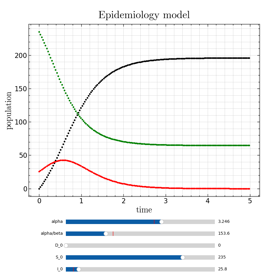

Estimating the α and β parameters for an epidemic

Although our equations cannot be easily solved as functions of time, it is possible to find out how I varies with S:

Thus, by using values of S and I from real-world epidemiological data, we can plot a y=mx graph and determine the line of best fit (via linear regression) whose gradient will best approximate α/β for our epidemic.

α can be found by running the model using a range of α values, and calculating the sum of square differences (SSD) between each iteration of the model and the real world data. The iteration with the lowest SSD value will have the optimal α value. Once α is found, since α/β is known (see above), β can be easily determined.

Where m denotes the m’th model run, evaluated using some unique value of α (the optimal value of α is between 2 and 4 for most epidemics).

For simplicity, we shall refer to α/β as rho from now on.

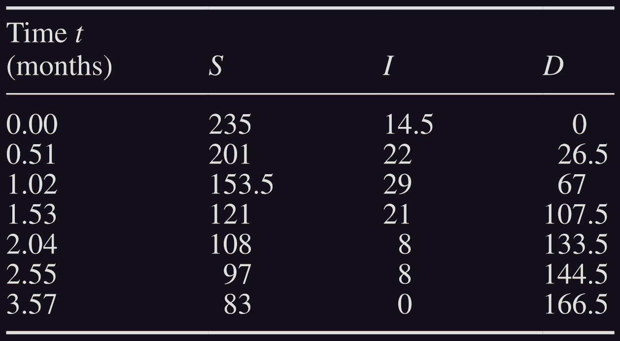
We shall use these ideas to model the Black Death using the data that William Mompesson (1639–1709) collected in the village of Eyam:

The python code used to calculate optimal alpha using SSD’s is shown below:

import matplotlib.pyplot as plt
            import numpy as np
            import scienceplots

            #linear regression for y=mx
            def lin_reg(x,y):
                return (x*y).mean(axis=0)/(x*x).mean(axis=0)

            #mompesson data
            t_momp = np.array([0,51,102,153,204,255,357])
            S_momp = np.array([235,201,153.5,121,108,97,83])
            I_momp = np.array([14.5,22,29,21,8,8,0])
            D_momp = np.array([0,26.5,67,107.5,133.5,144.5,166.5])

            #calculate rho = alpha/beta
            rho = lin_reg(np.log(S_momp[0]/S_momp),I_momp[0]+S_momp[0]-I_momp-S_momp)

            #create graph
            plt.style.use(['science','notebook'])

            fig, ax = plt.subplots(1,1, figsize=(10,10), dpi = 100)

            ax.grid(visible='yes',ls='--',lw=0.5,which='both')
            ax.set_title('Finding alpha by minimising SSD', fontdict = {'fontname':'CMU Serif','fontsize':25},y = 1.02)
            ax.set_xlabel('alpha', fontdict = {'fontname':'CMU Serif','fontsize':20})
            ax.set_ylabel('sum of square differences', fontdict = {'fontname':'CMU Serif','fontsize':20})

            #carry out calculations
            step = 1
            alpha = 2.5

            SSD_min = 1000
            alpha_min = 0

            while alpha < 3.5:
                SSD = 0
                beta = alpha/rho
                t = 0

                S_n = S_momp[0]
                I_n = I_momp[0]
                D_n = D_momp[0]

                while t < 400:
                    if t in t_momp:
                        index = np.where(t_momp == t)[0][0]
                        SSD += (S_n-S_momp[index])**2 + (I_n-I_momp[index])**2 + (D_n-D_momp[index])**2

                    del_D = alpha * I_n * step/100
                    del_S = - beta * S_n * I_n * step/100
                    del_I = (beta * S_n * I_n * step/100) - (alpha * I_n * step/100)
                    (D_n, S_n, I_n) = (D_n + del_D, S_n + del_S, I_n + del_I)
                    t += step
                
                if SSD < SSD_min:
                    SSD_min = SSD
                    alpha_min = alpha
                
                ax.plot(alpha,SSD,'r.')

                alpha += 0.005

            #create texbox showing rho, optimum alpha and minimised SSD
            note = '\n'.join(("rho = %.3f" % (rho), "lowest SSD = %.3f" % (SSD_min),"optimal alpha = %.3f" % (alpha_min)))
            ax.text(0.12,0.86,note,transform = ax.transAxes, bbox = dict(facecolor = 'w', edgecolor = 'k'), fontdict = {'fontname':'CMU Serif','fontsize':15})

            #show graph
            plt.show()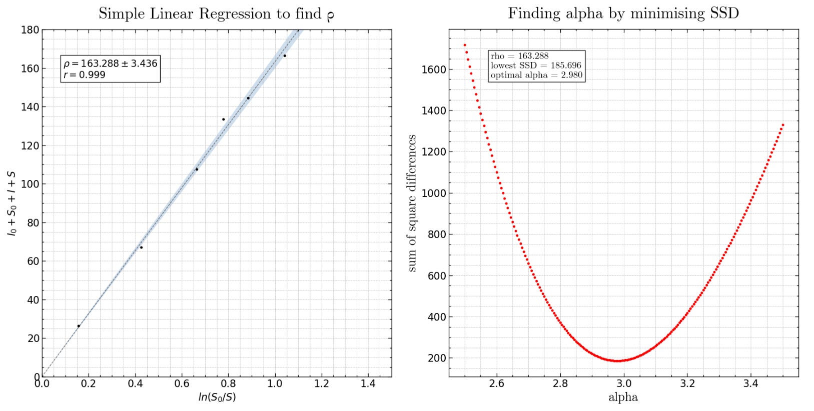

These values of rho and alpha can then be used as parameters to run our SIR model, and we can compare this with Mompesson’s data:

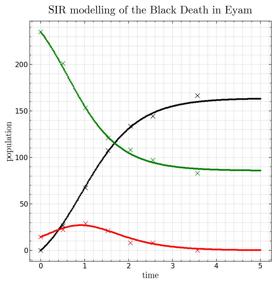
Pretty good!

The ups and downs of I

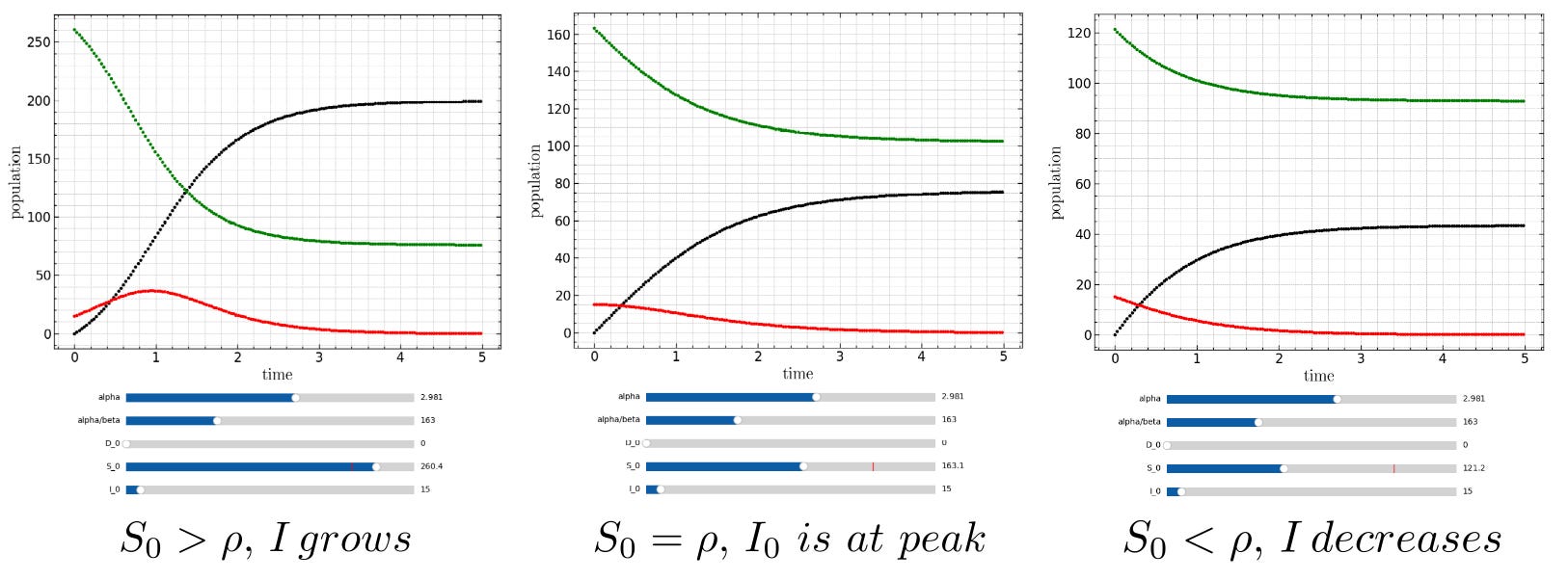
Recall that the equation for infectives is:

It is thus apparent that dI/dt = 0 if I = 0 or S = α/β (in other words, S = ρ). Taking the second derivative:

Thus we can see that I is at a maximum when S = ρ. This is the susceptible population at the peak of infection. ρ represent a threshold for the epidemic - if the susceptible population is below this value, the SIR model predicts that the number of infectives will reduce rather than grow.

Rewriting the SIR equations

The SIR equations become easier to solve if we rewrite them using a different set of variables. Since S_0 and β are unlikely to be known a priori, we will also use a different set of initial conditions.

We fit our curve around the peak of infection, (t_max, I_max), and extend time over a range of [-∞, ∞], rather than be constrained by some artificial point of data collection. We will also set our dead count to be 0 at the infection peak - this means that prior to the infection peak the dead count will be negative. This might all seem a bit bizarre but as you shall see it will simplify the math significantly, especially since S = ρ at the peak of infection.

Our new variables shall be:

And our initial conditions shall be:

where x_max = I_max / ρ.

Note that D(t = -∞) is the cumulative dead (+recovered) from the beginning of the model time to the peak of infection, which is a negative value.

Using our scaled variables, we can re-write the SIR equations as follows:

Extraordinary! Lets see how far we can take this…

The fixed population constraint means that:

Note that with τ = 0, z = 0, this means that the total population does not equal to ρ(x+y+z). With some careful thought we realise that it is:

Where z_ = D(t = -∞), which as we recall from the discussion above is a negative value. R₀ = N/ρ, is called the Basic Reproduction Number, which as we shall see later is a very important characteristic of an epidemic.

Solving SIR using a semi-analytic approach

We can use the above to express an equation for τ(z).

We get an integral expression which cannot be evaluated in a closed form sense. We could use a numerical method such as the trapezium rule. Alternatively, we can solve it by fitting a set of cubic splines to a vector of {z,f(z)} values and then evaluate the integral analytically:

It is clear from the form of f(z) that zero values of the denominator will cause an infinite asymptote. Since the denominator is x(z), and x = 0 when I = 0, i.e. the boundary values at (t = -∞, ∞), it is clear that the limits of z are the solutions to:

The limits of z, [z-, z+], can thus be found using the Newton-Raphson iterative numerical method:

The Newton-Raphson method will converge very rapidly to find a solution either side of a stationary point. Our stationary point is located at z = 0, thus we can run it with z(0) = 1 to get z+ and z(0) = -1 to get z-.

Thus, we can use the following steps to model an epidemic:

1. Input parameters ρ, α, I_max, t_max.

2. Find limits of z, [z-, z+], using the Newton-Raphson method.

3. Evaluate τ(z) by calculating the integral using a numerical method such as trapezium rule or cubic slice fitting + analytical integration.

4. Evaluate x(z) and y(z) using:

5. Determine S, I, D, t using:

6. Iterate z from z- to z+ and graph our values of S, I, D versus time.

Additionally:

• If the mortality fraction is known we can work out the fraction of D that are dead or recovered.

• We can also calculate the population size, N, and the Basic Reproduction Number, R₀ = N/ρ.

Solving SIR using the K&K approximation

Kermack and McKendrick proposed a time-symmetric-about-the-peak sech² approach to the SIR equations in the 19274 that became the standard until the criticism of Kendall in 19565.

The K&K approach uses the approximation (from the first three terms of the Mclaurin/Taylor expansion):

Which gives us:

For this to be valid, z«1, which means that the ratio of D to ρ must be smaller than 1 since z = [D + D(t = -∞)] / ρ. This means that as time goes on and more people die, the approximation will become increasingly inaccurate.

Under the K&K approximation, τ(z) becomes:

The final step makes use of the general integration result:

Rearranging for z gives us:

and therefore:

In summary, the K&K approximation to the SIR equations yields:

Since the limit of tanh(k) = ±1 as k approaches ±∞ :

Hence in the K&K approximation:

An implementation of the K&K approximation and its comparison to the Euler method in python is shown below:

import matplotlib.pyplot as plt
            import numpy as np
            import scienceplots

            #mompesson data
            t_momp = np.array([0,51,102,153,204,255,357])
            S_momp = np.array([235,201,153.5,121,108,97,83])
            I_momp = np.array([14.5,22,29,21,8,8,0])
            D_momp = np.array([0,26.5,67,107.5,133.5,144.5,166.5])
            t_max = 0.90
            I_max = 26.76

            #set parameters
            step = 0.005
            alpha = 2.98
            rho = 163
            beta = alpha / rho
            x_max = I_max / rho

            D_n = 0
            S_n = 235
            I_n = 14.5

            t = 0

            #graph setup
            plt.style.use(['science','notebook'])

            fig, axes = plt.subplots(1,2, figsize=(20,8), dpi = 100)

            ax = axes[0]
            ax.grid(visible='yes',ls='--',lw=0.5,which='both')
            ax.set_title('SIR model using Euler method and K&K approximation', fontdict = {'fontname':'CMU Serif','fontsize':20},y = 1.02)
            ax.set_xlabel('time', fontdict = {'fontname':'CMU Serif','fontsize':18})
            ax.set_ylabel('population', fontdict = {'fontname':'CMU Serif','fontsize':18})

            #plot euler method
            D_t = []
            S_t = []
            I_t = []
            t_t = []

            while t < 5:
                D_t.append(D_n)
                S_t.append(S_n)
                I_t.append(I_n)
                t_t.append(t)

                del_D = alpha * I_n * step
                del_S = - beta * S_n * I_n * step
                del_I = (beta * S_n * I_n * step) - (alpha * I_n * step)
                (D_n, S_n, I_n) = (D_n + del_D, S_n + del_S, I_n + del_I)
                t += step

            ax.plot(t_t,S_t,'g-',lw = 2, label = 'Euler S')
            ax.plot(t_t,I_t,'r-',lw = 2, label = 'Euler I')
            ax.plot(t_t,D_t,'k-',lw = 2, label = 'Euler D')

            #k&k approximation
            t = np.linspace(0,5,len(t_t))
            tau = alpha * (t-t_max)
            I_kk = rho*(x_max*np.cosh(((0.5*x_max)**0.5)*tau)**(-2))
            z = ((2*x_max)**0.5)*np.tanh(((0.5*x_max)**0.5)*tau)
            D_kk = rho*(z+(2*x_max)**0.5) - 33.06
            S_kk = rho*((np.e)**(-z))

            ax.plot(t,S_kk,'--',color = 'mediumaquamarine', label = 'K&K S')
            ax.plot(t,I_kk,'--',color = 'salmon', label = 'K&K I')
            ax.plot(t,D_kk,'--',color = 'purple', label = 'K&K D')

            #plot mompesson data
            ax.plot(t_momp/100,S_momp,'gx', markersize = 10, label = 'Mompesson S')
            ax.plot(t_momp/100,I_momp,'rx', markersize = 10, label = 'Mompesson I')
            ax.plot(t_momp/100,D_momp,'kx', markersize = 10, label = 'Mompesson D')

            #plot difference of euler and k&k
            ax = axes[1]
            ax.grid(visible='yes',ls='--',lw=0.5,which='both')
            ax.set_title('Comparing K&K approximation to Euler method', fontdict = {'fontname':'CMU Serif','fontsize':20},y = 1.02)
            ax.set_xlabel('time', fontdict = {'fontname':'CMU Serif','fontsize':18})
            ax.set_ylabel('Euler value - K&K value', fontdict = {'fontname':'CMU Serif','fontsize':18})

            ax.plot(t,S_t-S_kk,'g--',lw = 1.5, label = 'S')
            ax.plot(t,I_t-I_kk,'r--',lw = 1.5, label = 'I')
            ax.plot(t,D_t-D_kk,'k--',lw = 1.5, label = 'D')

            #show graph
            axes[0].legend(frameon=True, fontsize = 12, ncol = 3)
            axes[1].legend(frameon=True, fontsize = 12)
            plt.show()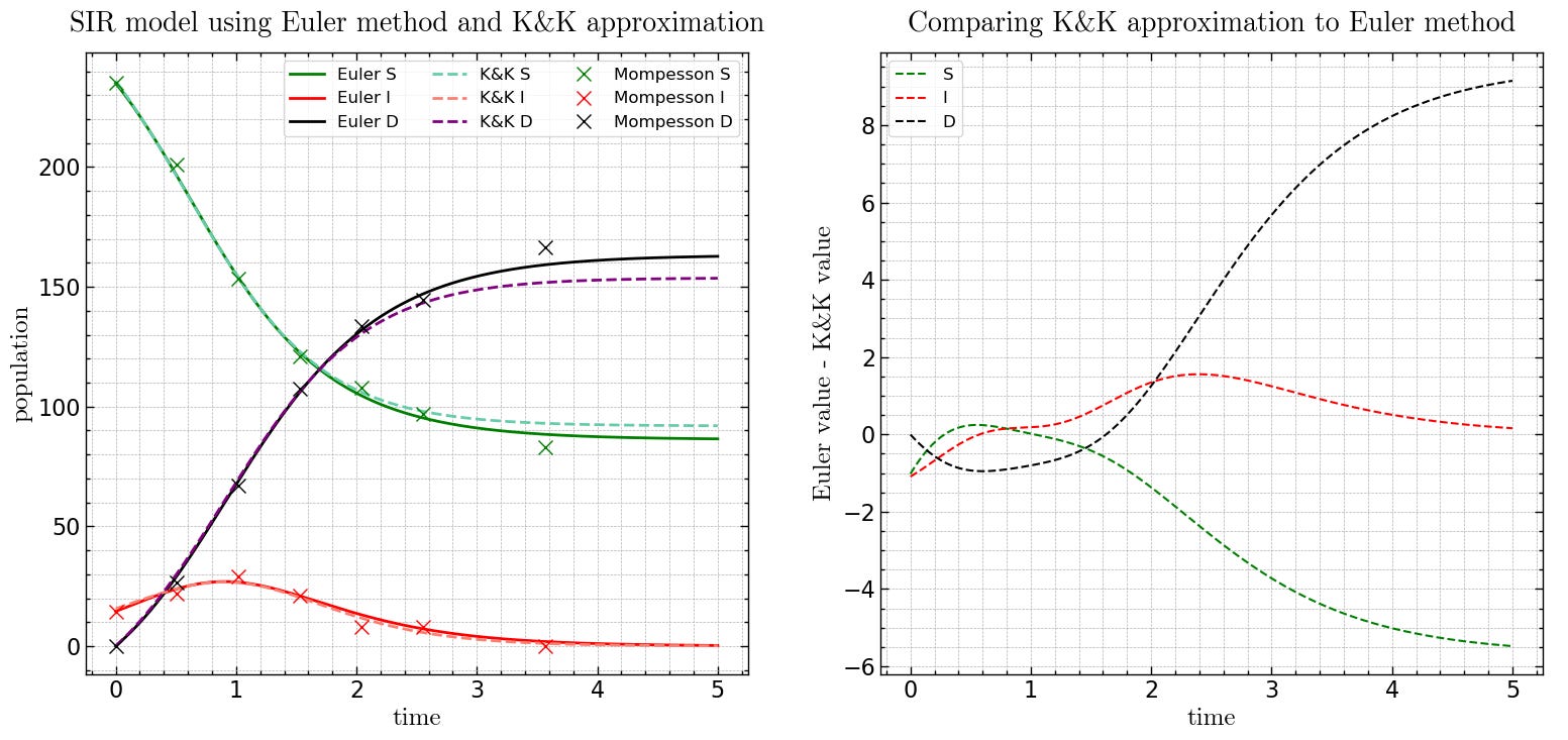

Using η instead of ρ

The semi-analytic and K&K approaches to the SIR model use inputs ρ, α, I_max, t_max. I_max and t_max can easily be estimated using epidemic data, and the range of α is relatively well bounded (between 2 and 4 for most epidemics, in units of month^(-1) ). The problem parameter is ρ, which can vary significantly: ρ=163 for Mompesson’s Black Death, ρ=1,538 for the 2014 Ebola epidemic in Liberia.

We can’t avoid having 4 inputs for the SIR model, but we can replace ρ with a different variable that has a much more well-defined range…

The total number of dead people is given by:

Clearly this cannot exceed the total population N, or be less than zero:

η must be in the range [0,1]. Recall that:

Therefore:

From our definition of η:

We can substitute this back into our expression for x=0 for positive z:

Thus:

If we start with η we don’t need to solve an iterative equation for z+ and z-, significantly reducing computation time.

Also, recall:

So, since we know I_max, we can easily find ρ:

Thus, we can follow an improved procedure for modelling our epidemic:

1. Input parameters η, α, I_max, t_max.

2. Calculate the limits of z using:

3. Calculate x_max and ρ using:

4. Evaluate τ(z) by calculating the integral using a numerical method such as trapezium rule or cubic slice fitting + analytical integration.

5. Evaluate x(z) and y(z) using:

6. Determine S, I, D, t using:

7. Iterate z from z- to z+ and graph our values of S, I, D versus time.

Additionally:

• If the mortality fraction is known we can work out the fraction of D that are dead or recovered.

• We can also calculate N and R₀:

The issue of finding optimal η and α still remains. We can implement an SSD method similar to the one we used earlier - we iterate the model using a range of η and α, plotting a 3D graph of SSD between the model and the real data, and the iteration at the minimum of the 3D surface will represent optimal values of η and α. In fact, we could compute SSD for ranges of all four input parameters, although this would be computationally expensive and it is hard to visualise a 5D graph.

I hope to write more posts on epidemiological modelling. Non-closed populations (N is not constant), vaccination and repeat illness are factors that need to be considered for most modern epidemics, and have not been accounted for in the above model. I would also like to implement a stochastic version of the SIR model utilising random probability distributions.

Notes